Basics

Pruning a model is the process of sparsifying the weight matrices within a model, thereby reducing its storage size by packing weights more efficiently. This can be done by setting a fraction of the values in the model’s weight matrices to zero.

Pruned weights can be represented more efficiently using a sparse representation rather than the typical dense representation. In a sparse representation, only non-zero values are stored, along with a bit mask, that takes the value 1 at the indices of the non-zero values. For example, if the weight values are

[0, 7, 0, 0, -3.2, 0, 0, 56.3]

the sparse representation contains a bit mask with 1s in the locations where the value is non-zero:

[0, 1, 0, 0, 1, 0, 0, 1]

This is accompanied by the non-zero data, which in the following example will look like:

[7, -3.2, 56.3]

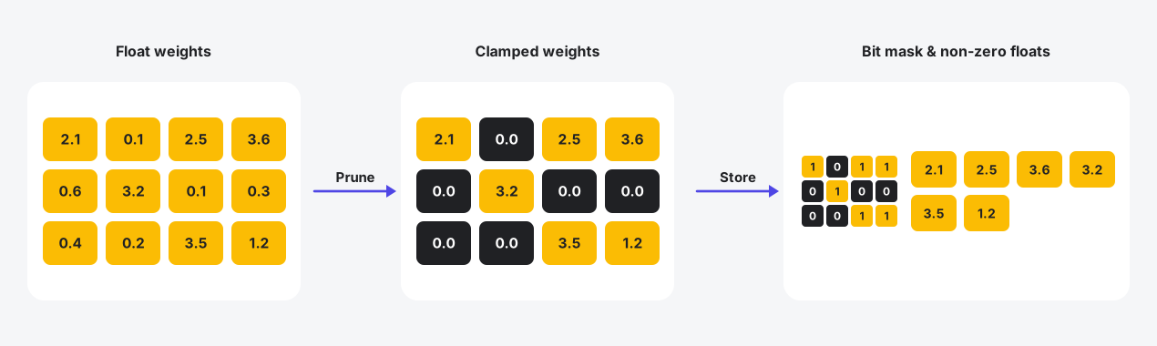
Magnitude pruning zeros out the smallest-magnitude weights and stores the result as a bit mask plus a packed list of non-zero values.

Pruning Algorithm

The pruning algorithm selects which elements to zero out.

• MagnitudePruning: A simple way to pick the elements to zero out is by the magnitude of the element. The magnitude pruner sorts the elements based on the value and zeros out the smallest set of elements up to the target_sparsity.

Pruning Schemes

Sparsity can be introduced either in an unstructured way (the 0s introduced follow no pattern) or in a structured way (0s will be grouped together based on a pattern). This can be configured using the PruningScheme.

• Unstructured: in this pruning scheme, there is no constraint for the 0s introduced into the tensor. For example, in the case of magnitude pruning with 50% sparsity, the pruner finds the smallest values in the tensor and zeros out half of them, wherever they may be located across the tensor.

• ChannelStructured: this pruning scheme constrains the 0s to entire channels (slices along a chosen axis of the tensor) — every element within a pruned channel is zeroed together. For example, in the case of magnitude pruning with 50% sparsity, channels are ranked by their L1 norm and the half with the smallest norms are zeroed out across all of their elements, while the other half are kept intact. The realized sparsity is rounded down to the nearest multiple of 1/num_channels.

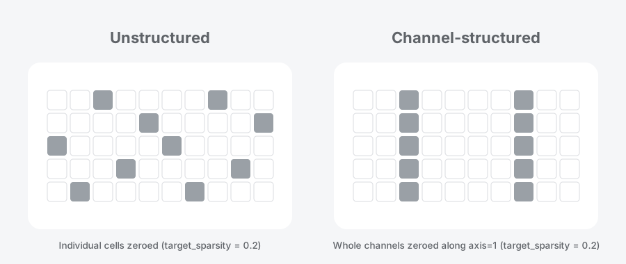
Unstructured pruning zeros individual cells anywhere in the tensor, while channel-structured pruning zeros entire channels together. Both reach the same overall 20% sparsity.

Pruning Schedule

When the sparsity is applied to the module, it introduces error into the module as a portion of the weight values are no longer contributing to the model’s output. In models that are sensitive to sparsity, it might help to apply the sparsity in an incremental manner while fine-tuning the model to adapt to the sparsification. The Pruning Schedule allows applying sparsity based on a certain schedule.

• ConstantSparsitySchedule: This is a simple schedule which mimics a step function. Up to begin_step the sparsity is 0%. Starting from begin_step, the schedule applies the entire target_sparsity to the model. This is a good first step to check how the model behaves with sparsity. For robust models and smaller amounts of sparsity, this works well and is recommended.

• PolynomialDecaySchedule: This schedule applies the sparsity based on a polynomial function which can be configured. The sparsity at step s within the schedule window is

sparsity(s) = s_target + (s_initial − s_target) · (1 − t)^power

where  t = (s − begin_step) / (total_iters − 1)

Starting from begin_step, the schedule incrementally applies the sparsity in increments of update_frequency up till the target_sparsity, following the polynomial described by the polynomial exponent power until total_iters is reached. Beyond total_iters, it will maintain the target_sparsity.

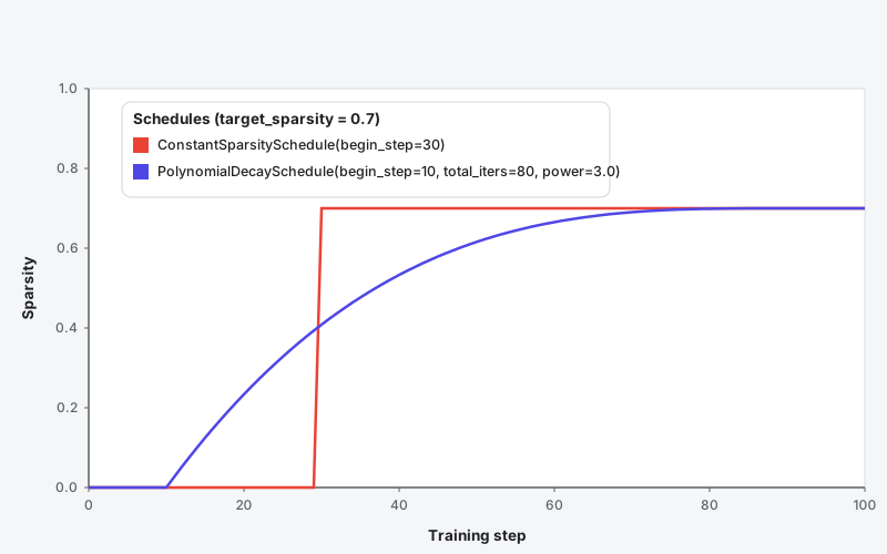
Sparsity over training steps under each schedule, both targeting 70% sparsity. The constant schedule jumps from 0% to the target at begin_step; the polynomial schedule ramps up smoothly with a slow start (power = 3) before plateauing at the target.